a) Compute the maintenance cost function based on the high-low method.
Step 1 Activity Cost
High 900 €2,500
Low 300 €1,800
Step 2 .Difference 600 €700
Step 3 €700 ¸ 600 = €1.17 (the variable cost per unit)
Step 4 Total cost = fixed costs + (variable cost per unit x number of units sold)
y = a + b(x)
2,500 = a + 1.17 (900)
2,500 = a + 1053
1,447 = a (the fixed cost amounts to €1,447)
Thus the cost function for maintenance as per the high-low method is y = 1,447 + 1.17(x)
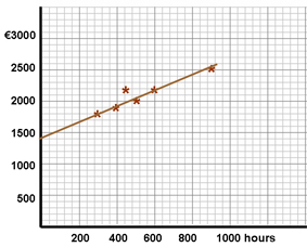
b)Draw a scatter diagram of the above data and draw a line of best fit through the data. From the graph, calculate the maintenance cost function.
c) Compute the maintenance cost function based on least squares regression analysis.
The calculations required to determine the total cost function for maintenance using least squares regression analysis are as follows:
|
Activity |
Cost € |
|
|
|
Month |
x |
y |
xy |
x2 |
y2 |
1 |
500 |
2,000 |
1,000,000 |
250,000 |
4,000,000 |
2 |
600 |
2,200 |
1,320,000 |
360,000 |
4,840,000 |
3 |
900 |
2,500 |
2,250,000 |
810,000 |
6,250,000 |
4 |
400 |
1,900 |
760,000 |
160,000 |
3,610,000 |
5 |
300 |
1,800 |
540,000 |
90,000 |
3,240,000 |
6 |
450 |
2,000 |
900,000 |
202,500 |
4,000,000 |
|
3,150 |
12,400 |
6,770,000 |
1,872,500 |
25,940,000 |
|
|
|
|
|
|
The linear regression equation, which meets the above requirement, is obtained from solving simultaneously two equations. This gives us values for both a (fixed costs) and b (variable cost per unit) in the total cost function. The equations are as follows
1. å y = na + b åx 2. åxy = a(åx) + b åx2 a = fixed cost, b = variable cost per unit, n = number of observations, åx = Sum of the observations of the independent variable, åy = Sum of the observations of the dependant variable, åxy = Sum of the product of each pair of observations and åx2 = Sum of the squares of the x observations. |
Equation 1 12,400 = 6a + b3150
Equation 2 6,770,000 = a3,150 + b1,872,500
By multiplying equation 1 by 525 we bring the number of (a)’s to the same number in each equation and thus cancel the (a) variable.
Equation 1 6,510,000 = a3,150 + b1,653,750
Equation 2 6,770,000 = a3,150 + b1,872,500
Subtract equation 1 from equation 2
260,000 = b218,750
1.19 = b
Substituting 1.19 for (b) in equation 1 should give us a value for (a)
12,400 = 6a + 1.19(3,150)
12,400 = 6a + 3,748.5
8,651.5 = 6a
1,442 = a
Thus according to the least squares regression method the repairs and maintenance costs for the leisure centre show a fixed element of €1,442 and a variable element of €1.19 per person or user.
d) Outline the main reasons for the differences in the maintenance cost function calculated by each of the methods.
As can be seen below, each method will give a different cost function.
1. High-low Y = 1,447 + 1.17(x)
2. Scatter-graph Y =
3. Linear regression Y = €1,442 + €1.19 (x)
The main reasons for the different cost functions are connected to the limitations of each approach. For example the main limitation of the high-low method is that the two sets of data selected may not be representative of the real behaviour patterns of the costs. For example, the highest and lowest activities may have occurred during exceptional circumstances and hence this method can provide a misleading cost function.
The main difference between the scatter-graph and high-low method lies with the sample data used to ascertain the cost function. The scatter-graph approach uses all the data in the sample to estimate the line of best fit and hence the cost-function. The high-low method uses only two extreme points within the sample to estimate the cost function. The main weakness of the scatter-graph approach is that once all the data is plotted on a graph, deciding on a line of best fit is still a subjective judgement.
Of the three methods, the linear regression model is considered to have the least number of limitations. This method is a statistical approach to determine the line of best fit for a given set of data. It is an extension of the scatter-graph approach and is based on the principle that the sum of the squares of the vertical distances from the regression line to the plots of the data points is less than the sum of the squares of the vertical distances from any other line that may be determined. In other words a truly objective line of best fit is calculated which minimises the squared deviations between the regression line and the observed data.
e) What is the advantage in calculating a cost function for a cost item?
The cost function can be used in the intelligent prediction of future costs based on forecast sales activity. This can provide more accurate forecast cost information which supports management planning and decision-making